38 how to add labels to pie chart in excel
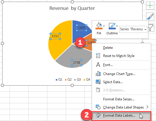
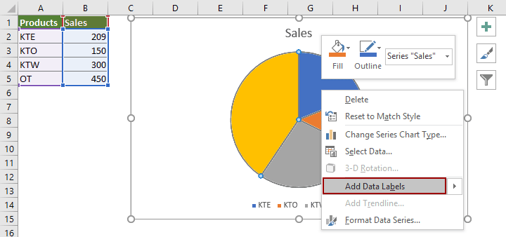
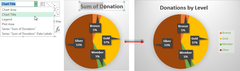
Change the format of data labels in a chart - Microsoft Support To get there, after adding your data labels, select the data label to format, and then click Chart Elements > Data Labels > More Options. To go to the appropriate area, click one of the four icons ( Fill & Line, Effects, Size & Properties ( Layout & Properties in Outlook or Word), or Label Options) shown here. Pie Chart in Excel | How to Create Pie Chart - EDUCBA Guide to Excel Pie Chart. Here we discuss how to use Pie Chart in Excel along with practical examples and downloadable excel template. EDUCBA. MENU MENU. ... Step 10: Now, right-click on one of the slices of the pie and select add data labels. This will add all the values we are showing on the slices of the pie. Step 11: ...
How can I change label sizes & shapes in Excel pie charts? Jun 28, 2011 · When I create a pie chart in Excel (2007), often I would like to change the overall size of the data labels but Excel does not seem to allow this. I have tried clicking on the corners of the label ...
How to add labels to pie chart in excel
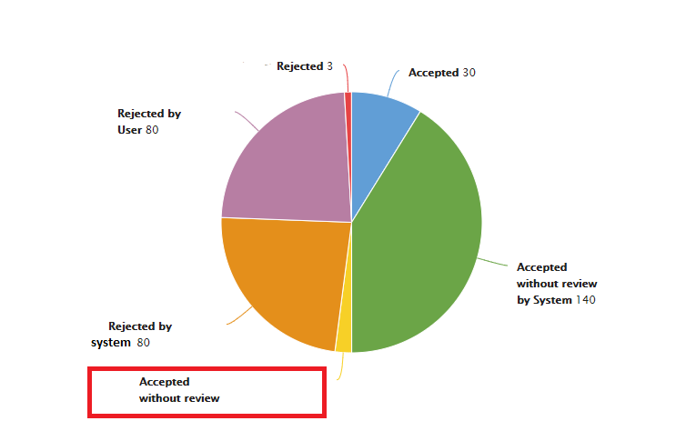
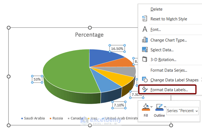
How to display leader lines in pie chart in Excel? - ExtendOffice To display leader lines in pie chart, you just need to check an option then drag the labels out. 1. Click at the chart, and right click to select Format Data Labels from context menu. 2. In the popping Format Data Labels dialog/pane, check Show Leader Lines in the Label Options section. See screenshot: How to insert data labels to a Pie chart in Excel 2013 - YouTube This video will show you the simple steps to insert Data Labels in a pie chart in Microsoft® Excel 2013. Content in this video is provided on an "as is" basi... How to Edit Pie Chart in Excel (All Possible Modifications) Feb 19, 2023 · Steps: Firstly, click on the chart area. Following, go to the Chart Design tab on the ribbon. Subsequently, click on the Switch Row/Column tool. Therefore, you can switch the row and column of your pie chart. Read More: How to Edit a Macro Button in Excel (5 Easy Methods) 11. Explode Individual Category of a Pie Chart.
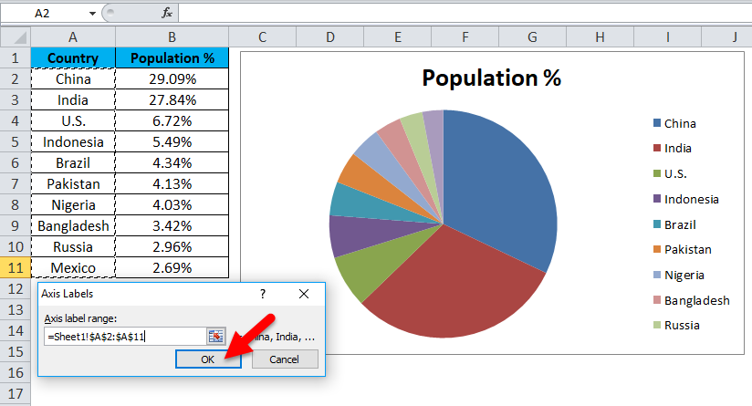
How to add labels to pie chart in excel. Excel Pie Chart Labels on Slices: Add, Show & Modify Factors -... Feb 7, 2023 · The method to add category names to the data labels is given below step-by-step: 📌 Steps: First, double-click on the data labels on the pie chart. As a result, a side window called Format Data Labels will appear. Now, go to the drop-down of the Label Options to Label Options tab. Then, check the Category Name option. How to Edit Pie Chart in Excel (All Possible Modifications) Feb 19, 2023 · Steps: Firstly, click on the chart area. Following, go to the Chart Design tab on the ribbon. Subsequently, click on the Switch Row/Column tool. Therefore, you can switch the row and column of your pie chart. Read More: How to Edit a Macro Button in Excel (5 Easy Methods) 11. Explode Individual Category of a Pie Chart. How to insert data labels to a Pie chart in Excel 2013 - YouTube This video will show you the simple steps to insert Data Labels in a pie chart in Microsoft® Excel 2013. Content in this video is provided on an "as is" basi... How to display leader lines in pie chart in Excel? - ExtendOffice To display leader lines in pie chart, you just need to check an option then drag the labels out. 1. Click at the chart, and right click to select Format Data Labels from context menu. 2. In the popping Format Data Labels dialog/pane, check Show Leader Lines in the Label Options section. See screenshot:
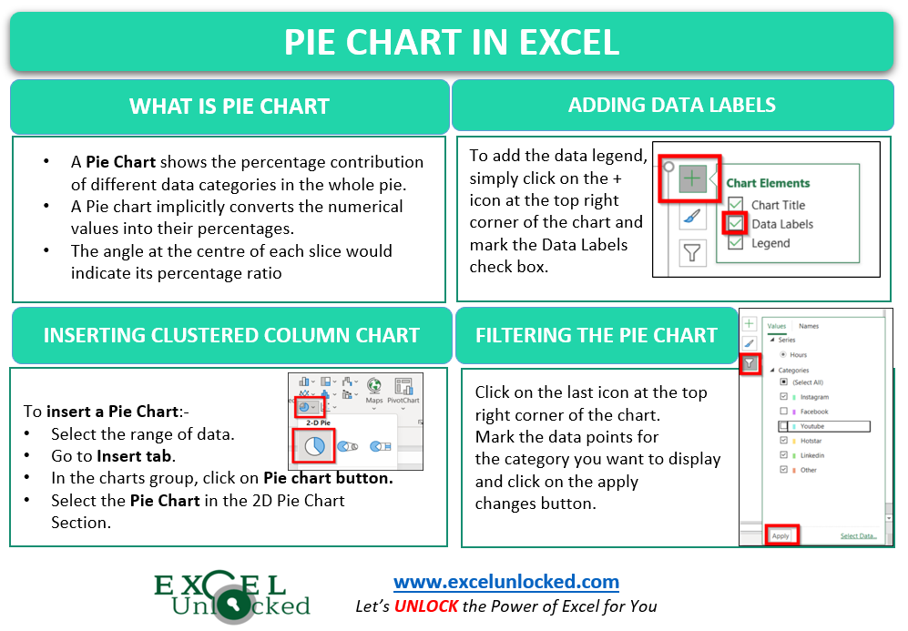
Pie Chart in Excel - Inserting, Formatting, Filtering - Excel ...

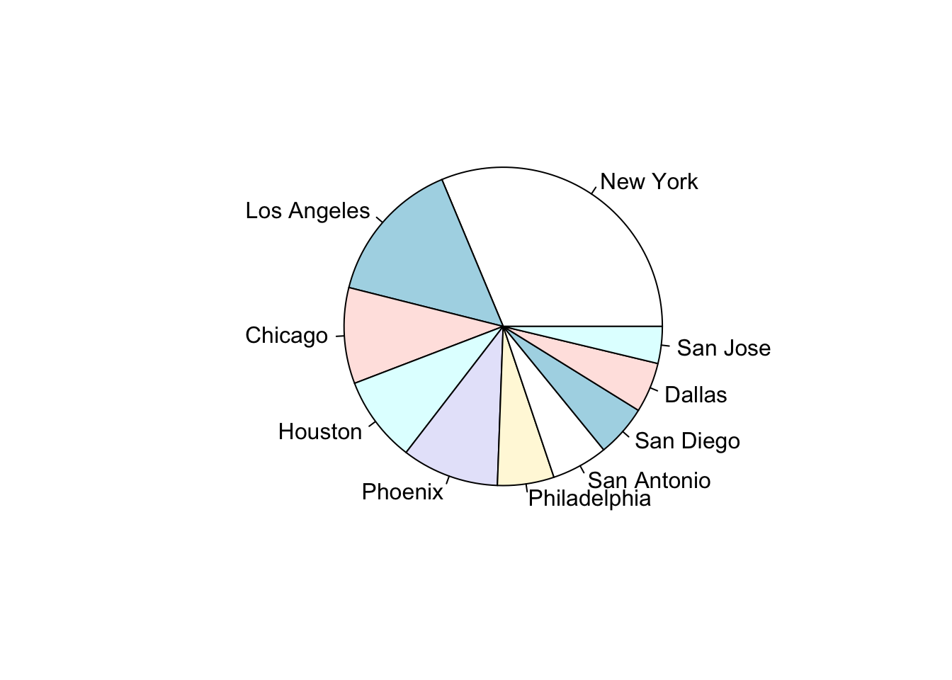
Interactive R pie chart labels. Statistics for Ecologists ...
Pie Chart - Show Percentage - Excel & Google Sheets ...
Chapter 9 Pie Chart | Basic R Guide for NSC Statistics

Microsoft Excel Tutorials: Add Data Labels to a Pie Chart
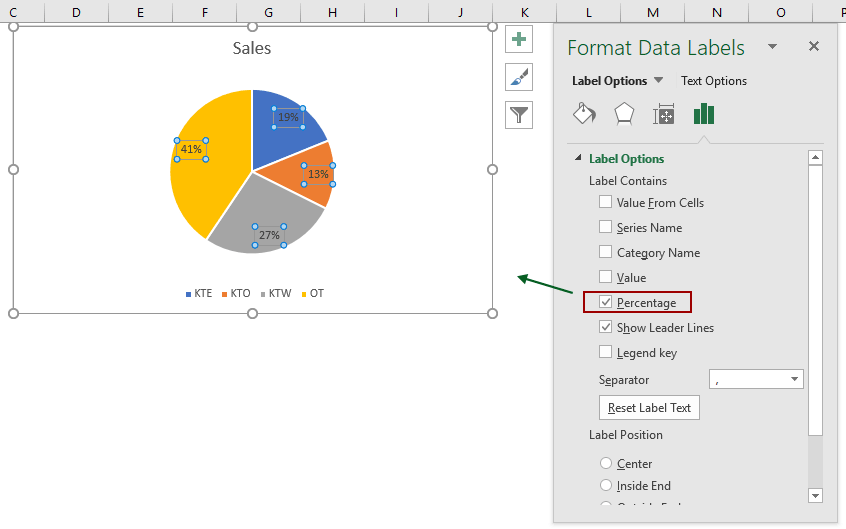
How to show percentage in pie chart in Excel?

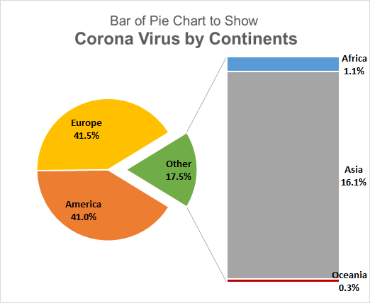
How to Create Bar of Pie Chart in Excel Tutorial!

Excel Pie Chart Good Bad Examples Videos ◔ - Contextures
How to Create a Pie Chart in Excel | Smartsheet

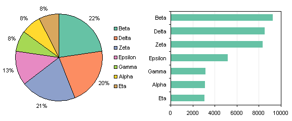
Automatically Group Smaller Slices in Pie Charts to one big Slice
How-to Make a WSJ Excel Pie Chart with Labels Both Inside and ...
How to make an Excel pie chart with percentages
Excel Doughnut chart with leader lines – teylyn

How to Show Percentage in Pie Chart in Excel? - GeeksforGeeks

How to data label on pie chart? - Simple Excel VBA
Appian Community
How to Show Pie Chart Data Labels in Percentage in Excel
How to show percentage in pie chart in Excel?

How to fix wrapped data labels in a pie chart | Sage Intelligence
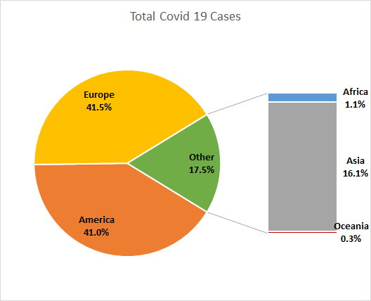
When to Use Bar of Pie Chart in Excel
Excel Doughnut chart with leader lines – teylyn
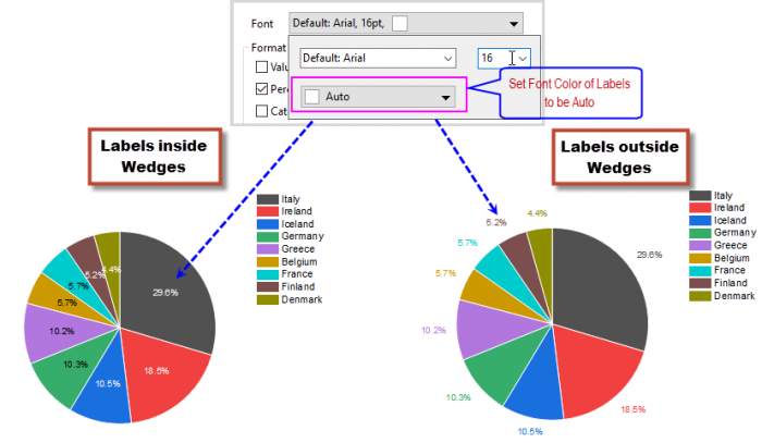
Help Online - Quick Help - FAQ-1019 How to customize the font ...
Pie Chart Rounding in Excel - Peltier Tech
Pie Charts bring in Best Presentation for Growth

How-to Add Label Leader Lines to an Excel Pie Chart - Excel ...

Change color of data label placed, using the 'best fit ...

How to Create a Pie Chart in Excel | Smartsheet
Add Labels with Lines in an Excel Pie Chart (with Easy Steps)

Add or remove data labels in a chart - Microsoft Support

How to Change Excel Chart Data Labels to Custom Values?

Excel: How to not display labels in pie chart that are 0 ...
Create a Pie Chart in Excel (Easy Tutorial)
Create Outstanding Pie Charts in Excel | Pryor Learning

Optimally positioning pie chart data labels in Excel with VBA ...

Create Outstanding Pie Charts in Excel | Pryor Learning
Pie Chart in Excel | How to Create Pie Chart | Step-by-Step ...
How to Create Bar of Pie Chart in Excel? Step-by-Step

How-to Add Label Leader Lines to an Excel Pie Chart
Post a Comment for "38 how to add labels to pie chart in excel"